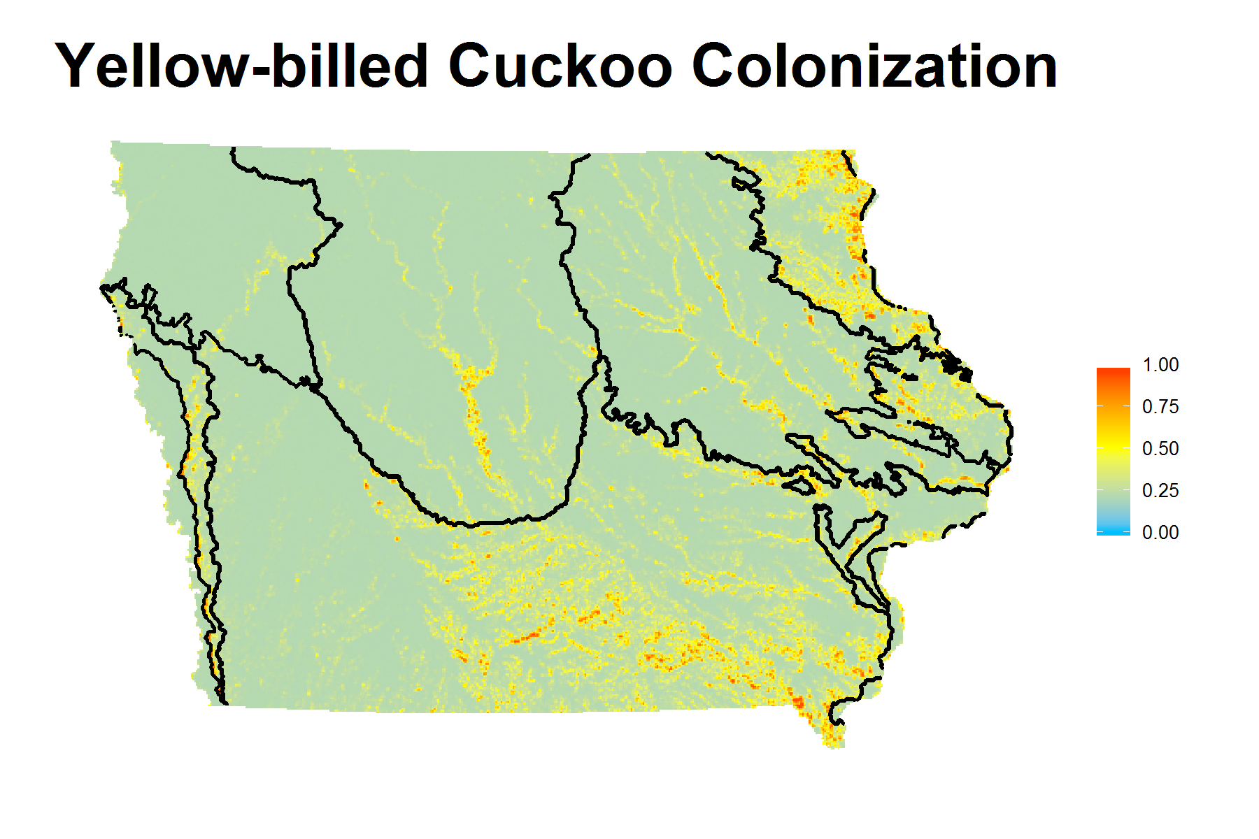
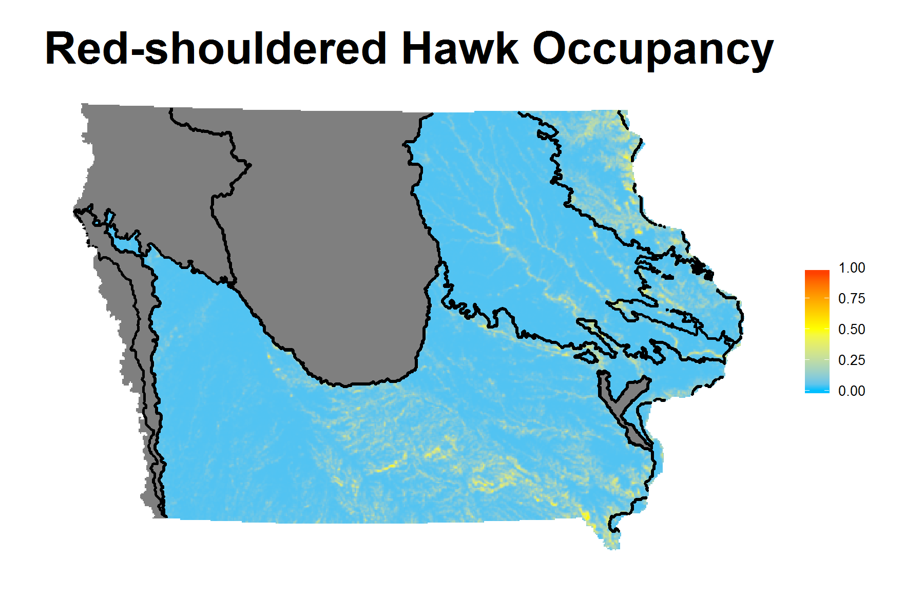
class: center, middle, inverse, title-slide # Shiny Application to Iowa DNR MSIM-SGCN Modeling ### Xiaodan (Annie) Lyu ### Join work with Tyler M. Harms ### September 23, 2016 --- ## Introduction - Period: Oct 2015 - May 2016 - State Wildlife Grants - Iowa Department of Natural Resources - Run predictive models using R package RMark - Produce predictive maps using ArcGIS - Develop an interactive web application using Shiny --- ## Outline - Project overview: data source and objectives - Methods: model fit and covariates - Model Validation: AUC - Results: example of estimates table and predictive maps - Demonstrate Shiny application --- ## Data Collection - Multiple Species Inventory and Monitoring (MSIM) Program + Iowa DNR and Iowa State University - Sampling Interval + Primary: 2006-2014 + Secondary: survey occasions (days) - Survey Objects + 414 SGCN, only 69 SGCN where sufficient data were available + Birds, mammals, reptiles, amphibians, odonates and butterflies --- ## Objectives - Predict the distribution of species of conservation need + robust design occupancy model - Create predictive species maps for priority SGCN + ArcGIS raster files + Shiny interactive web application - Prioritize areas of conservation action for SGCN + habitat restoration and management --- ## Methods - Robust design occupancy model (MacKenzie et al. 2003) + package RMark - Parameters of Interest + probability of occupancy ( `\(\psi\)` ) + probability of colonization ( `\(\gamma\)` ) + probability of extinction ( `\(\epsilon\)` ) + probability of detection ( `\(p\)` ) - Model types + RDOccupEG, RDOccupPE, RDOccupPG, ... --- ## Statistical Model `$$Pr(\mathbf{X}_i) = \boldsymbol{\phi}_0 \Bigg\{\prod_{t=1}^{T=1}D(\mathbf{p}_{X,t})\boldsymbol{\phi}_t \Bigg\} \mathbf{p}_{X,T}$$` - `\(\mathbf{p}_{X,t}\)` : vector denoting probability of observing the detection history `\(X_{i,t}\)` in primary period `\(t\)` - `\(\boldsymbol{\phi}_t\)` : matrix of transition probabilities between states of occupancy from primary period `\(t\)` to `\(t+1\)` `$$\begin{aligned} \boldsymbol{\phi}_t &= \begin{bmatrix} P(X_{t+1}=1|X_t=1) & P(X_{t+1}=0|X_t=1) \\ P(X_{t+1}=1|X_t=0) & P(X_{t+1}=0|X_t=0) \end{bmatrix} \\ &= \begin{bmatrix} 1-\epsilon_t & \epsilon_t \\ \gamma_t & 1-\gamma_t \end{bmatrix}, t = 1, ..., \text{T-1} \end{aligned}$$` `$$\phi_0 = \begin{bmatrix} \psi_1 & 1-\psi_1 \end{bmatrix}$$` --- ## Example `$$\begin{aligned} Pr(\boldsymbol{X}_{i,1} = 010) &= \psi_1(1-p_{1,1})p_{1,2}(1-p_{1,3}) \\ Pr(\boldsymbol{X}_{i,2} = 000|\boldsymbol{X}_{i,1}) &= (1-\epsilon_1)\prod_{j=1}^3(1-p_{2,j})+\epsilon_1 \\ Pr(\boldsymbol{X}_i = \text{010 000}) &= \phi_0 D(\boldsymbol{p}_{010,1}) \phi_1 \boldsymbol{p}_{000,2} \\ &= \begin{bmatrix} \psi_1 & 1-\psi_1 \end{bmatrix} \begin{bmatrix} (1-p_{1,1})p_{1,2}(1-p_{1,3}) & 0 \\ 0 & 0 \end{bmatrix} \\ &\ \ \ \times \begin{bmatrix} 1-\epsilon_1 & \epsilon_1 \\ \gamma_1 & 1-\gamma_1 \end{bmatrix} \begin{bmatrix} \prod_{j=1}^3(1-p_{2,j}) \\ 1 \end{bmatrix} \\ &= \psi_1(1-p_{1,1})p_{1,2}(1-p_{1,3})\Big[(1-\epsilon_1)\prod_{j=1}^3(1-p_{2,j})+\epsilon_1\Big]\end{aligned}$$` --- ## Statistical Model (cont'd) - Including Covariates `$$\theta = \frac{\exp(\boldsymbol{Z'\beta})}{1+\exp(\boldsymbol{Z'\beta})}$$` + `\(\theta\)` is the probability of interest + `\(\mathbf{Z}\)` is the matrix of covariate information + `\(\boldsymbol{\beta}\)` is the vector of logistic model coefficients to be estimated --- ## Covariates - Landscape habitat variables <sup>[1]</sup> + Radius of sampled site: 200m, 500m and 1km + Land use classification: Water, Wetland, Grassland, Woodland and Agriculture + Landscape configuration: percentage of landscape (PLAND), large patch index (LPI), edge density (ED), patch density (PD) and interspersion-juxtaposition (IJI) - Climate variables <sup>[2]</sup> + Wind speed (km/h), Cloud cover (%), Temperature ( `\(^\text{o}\text{C}\)` ) .footnote[ [1] site-specific, modeled on `\(\psi, \gamma\)` and `\(\epsilon\)` [2] time-varying, modeled on `\(p\)` ] --- ## Model Selection and Validation - Akaike's Information Criterion adjusted for small sizes ( `\(\text{AIC}_c\)` ) + Models with `\(\Delta \text{AIC}_c \leq 2 \Rightarrow\)` strong support (Burnham and Anderson 2002) - Area under the receiver operating characteristic curve (AUC) + evaluate performance of predicting occupancy + training data set: survey years 2006-2012, 2014 + test data set: survey year 2013 (better representative) + package pROC + `\(\text{AUC} = 0.5 \Rightarrow\)` random guess + `\(\text{AUC} = 1.0 \Rightarrow\)` perfect prediction (Jimenez-Valverde 2012) --- ## ROC Curve <img src="IDNR_SWG_16fall_files/figure-html/unnamed-chunk-1-1.png" style="display: block; margin: auto;" /> --- ## Results Results Summary | Statistics | Value/Range | | --------------------------------- | -------- | | Number of SGCN modeled | 64 out of 69 | | Occupancy Prob `\(\hat\psi\)` | 0.001(0.0003)~0.995(0.004) | | Colonization Prob `\(\hat\gamma\)` | 0.0003(0.0001)~0.999(0.00007) | | Detection Prob `\(\hat p\)` | 0.030(0.028)~0.998(0.006) | | AUC values | 0.426~0.921 | | Number of `\(\text{AUC} > 0.5\)` | 61 out of 64 | --- ## Results (Cont'd) Best Models for Each Specie |Species |Model | |:-------------------------------------------|:------------------------------| |Red-shouldered Hawk | `\(\psi\)`(Wod1KPLND) `\(\gamma\)`(Ag1KPD)p(Cld) | |Yellow-billed Cuckoo | `\(\psi\)`(Wod500PLND) `\(\gamma\)`(Wod1kLPI)p(Wind) | |Red-headed Woodpecker | `\(\psi\)`(Wod500PLND) `\(\gamma\)`(Ag500PD)p(Cld) | |Eastern Wood-pewee | `\(\psi\)`(Wod500PLND) `\(\gamma\)`(Wod1KPLND)p(Wind) | |Acadian Flycatcher | `\(\psi\)`(Wod500PLND) `\(\gamma\)`(Wod500PLND)p(Wind) | |Veery | `\(\psi\)`(Wod1kED) `\(\gamma\)`(Ag500LPI)p(Wind) | --- ## Results (Cont'd) AUC and Coefficients Estimates under Best Model <div id="htmlwidget-8fd921e38377382f6429" style="width:100%;height:auto;" class="datatables html-widget"></div> <script type="application/json" data-for="htmlwidget-8fd921e38377382f6429">{"x":{"filter":"none","data":[["1","2","3","4","5","6"],["Red-shouldered Hawk","Yellow-billed Cuckoo","Red-headed Woodpecker ","Eastern Wood-pewee","Acadian Flycatcher","Veery"],[0.7982,0.7062,0.6101,0.9059,0.8919,0.5506],[0.034433,0.059609,0.016901,0.1279653,0.0917458,0.005458],[0.002018,0.042017,-0.0023,0.0706042,0.0696241,-0.57778],[-0.00802,-0.07574,-0.00429,-0.1098943,0.0861607,0.178889]],"container":"<table class=\"display\">\n <thead>\n <tr>\n <th> <\/th>\n <th>Species<\/th>\n <th>AUC<\/th>\n <th>Psi.Cov<\/th>\n <th>Gam.Cov<\/th>\n <th>p.Cov<\/th>\n <\/tr>\n <\/thead>\n<\/table>","options":{"dom":"t","columnDefs":[{"className":"dt-right","targets":[2,3,4,5]},{"orderable":false,"targets":0}],"order":[],"autoWidth":false,"orderClasses":false,"rowCallback":"function(row, data) {\nDTWidget.formatRound(this, row, data, 2, 3, 3, ',', '.');\nDTWidget.formatRound(this, row, data, 3, 3, 3, ',', '.');\nDTWidget.formatRound(this, row, data, 4, 3, 3, ',', '.');\nDTWidget.formatRound(this, row, data, 5, 3, 3, ',', '.');\n}"}},"evals":["options.rowCallback"],"jsHooks":[]}</script> ---  ---  --- ## Shiny - **Shiny** by RStudio is a web application framework for R. - No HTML, CSS or JavaScript knowledge required to turn your analyses into interactive web applications. ```r install.packages("shiny") library("shiny") runExample("01_hello") ``` - ui.R defines the page layout and user interface - server.R contains the R code to create any output - More information available at [Shiny Webpage](http://shiny.rstudio.com/) --- ## About Our Shiny Application - Interactive web application to display predictive maps and parameter estimates for each SGCN - Easy to download personalized data and maps - Available to researchers and managers across Iowa (credentials needed) - Hosted by CSSM for 1-2 years - The URL for accessing the application is [https://dnrswg.cssm.iastate.edu/](https://dnrswg.cssm.iastate.edu/)